

PyFinPO - Python Financial Portfolio Optimization Library
PROJECTS · QUANTITATIVE FINANCE

Quant Finance, Portfolio Optimization

450h

Jan. 2024 - Present
INTRO
Project Description
Welcome to PyFinPO, my personal library for Financial Portfolio Optimization in Python.
PyFinPO is a simplified abstraction of other Python libraries for Portfolio Optimization (PyPortOpt, skfolio, scikit-learn, cvxpy...), aiming to provide a structured, direct and extensible infrastructure to perform Financial Portfolio Optimization.
SKILLS
Fields of Expertise
Quantitative Research:
Portfolio Optimization:
Asset Forecasting/Prediction (Expected Return Models, Risk Models…):
Coding (Python):
· · ·
Complexity: ★★★★★
Tools: Python
Project Type: Personal Project


01
Introduction __________
Project Introduction
Chapter 1 -
__ INTRO
When I first set out to develop a Portfolio Optimization Library in Python, my goal was simple: to gain a deep understanding of portfolio theory and its main methods. Building everything from scratch felt like the best way to learn the nuances of the different models, approaches, estimators... and their implementations.
However, as I started exploring the existing Portfolio Optimization libraries in Python, I discovered that there are already VERY GOOD resources available for free (see list below). I quickly came to the realization that it made no sense to implement my own portfolio tool from scratch having all those open-source libraries available –tested and improved through user feedback– that already included most of the Portfolio Optimization tools needed. Reinventing the wheel no longer seemed practical or efficient.
So I changed my mind. Instead of creating yet another standalone library, I decided that in order to understand the nuances of Portfolio Optimization, it would make more sense for me to build a centralized library which organizes the different functionalities available in other open-source libraries under a single, cohesive API. By integrating their strengths with an intuitive high-level interface, this tool could help me (and potentially other users) to seamlessly access the best functionalities each library has to offer without needing to master multiple APIs.
Additionally, I decided to prioritize modularity and extensibility, making extremely easy to add new proprietary models and integrate them in the buit-in API with minimal effort.
In a nutshell, I defined 3 main principles for the project: unified structure, intuitive use, and scalable modularity.
__ INTRO
Unified PO
Functionalities
Intuitive Use

To unify the different Portfolio Optimization functionalities offered in other libraries under a common, structured API.
To provide an intuitive, high-level interface to perform Portfolio Optimization with Python.
Scalable Modularity
To offer a MODULAR and EXTENSIBLE tool which anyone can use to build proprietary models and feed them into the created API structure to leverage the already implemented functionalities in existing libraries.
Project
Motivation
Project
Objectives
02
Content __________
Content & Structure
Chapter 2 -
Content
03
Features __________
PyFinPO Features
Chapter 3 -
___ PYFINPO FEATURES
Overview of
Portfolio Optimization Problem
Portfolio optimization, as formalized by Harry Markowitz in his seminal 1952 paper "Portfolio Selection," revolutionized investment theory by introducing a systematic and quantitative framework to allocate capital among all the available assets. Markowitz demonstrated that by combining securities with differing expected returns and volatilities, investors can construct portfolios that either minimize risk for a given return or maximize return for a specific level of risk. These optimal portfolios form the efficient frontier, a cornerstone of what is now known as Modern Portfolio Theory (MPT).
At the heart of Markowitz’s framework is mean-variance optimization, which requires two key inputs: estimates of expected returns and a covariance matrix to capture asset interdependencies. While the model provides a theoretically optimal solution, its practical application is limited by the difficulty in accurately forecasting these inputs. Historical data is often used as a proxy, though this approach sacrifices the theoretical guarantees of precision.
Advancements in portfolio optimization have expanded upon these ideas, introducing diverse objective functions and measures of risk such as maximizing Sharpe ratios or minimizing Conditional Value at Risk (CVaR). Constraints such as budget limits, sector exposure, or regulatory requirements are incorporated to reflect real-world considerations.
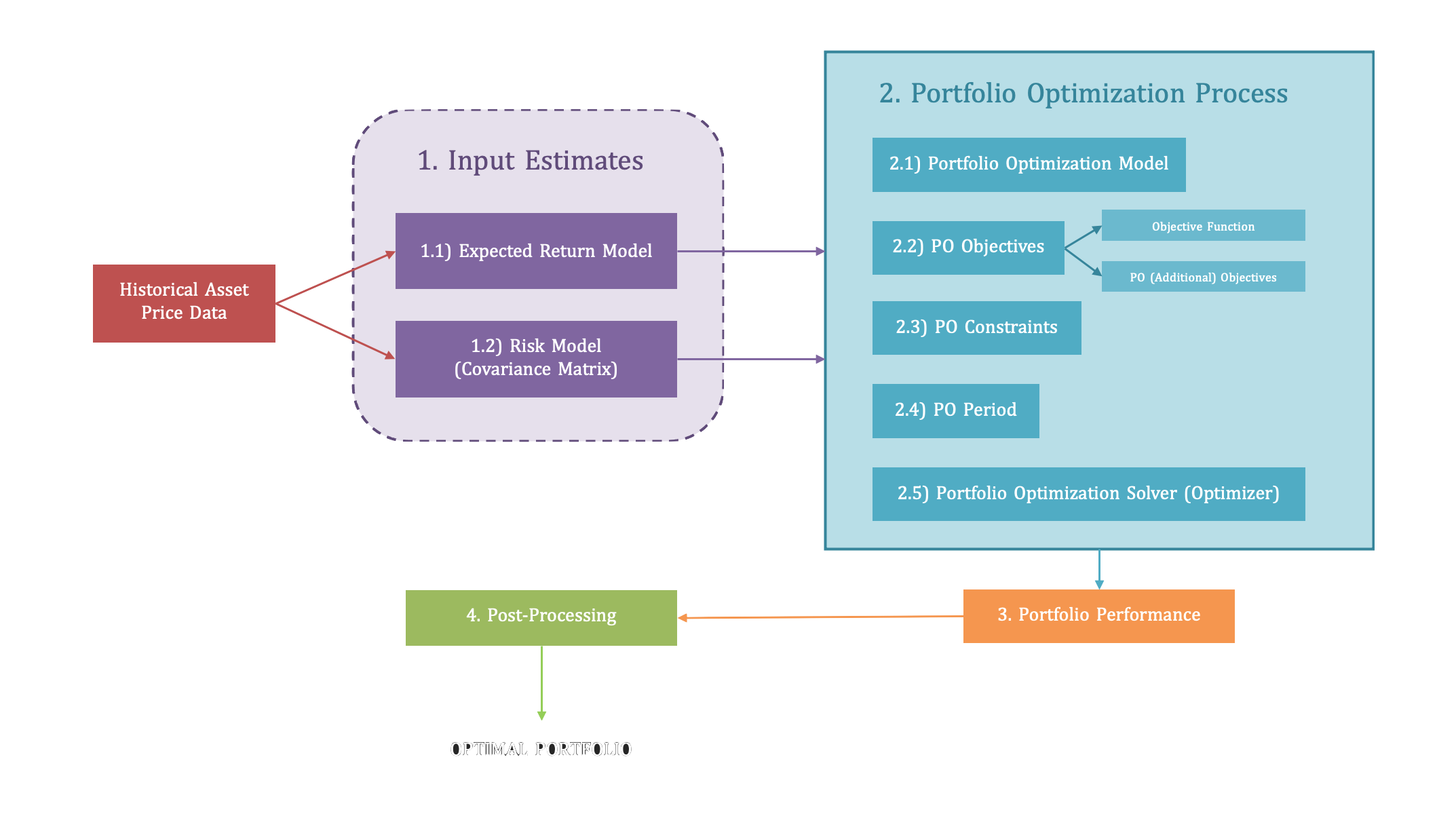
Building from the basic steps of Portfolio Optimization Theory, we can divide portfolio optimization process in 4 main steps, each with their own sub-steps. These are depicted in the Figure below, and fully detailed in the following section.
Four Features.
One Single Library.
1
3
__ Feature I
Input
Estimates
Input estimates aim to forecast the expected return and risk of portfolio securities, to be used as inputs for portfolio optimization.
__ Feature III
__ Feature II
Portfolio
Optimization
Once the input estimates are determined, we can proceed with the portfolio optimization process, which is divided in 5 main steps.
__ Feature IV
Portfolio
Post-Processing
Finally, with the Portfolio Post-Processing module we can generate portfolio outputs and graphics in a user-friendly format.
Portfolio
Performance
Once an optimal portfolio is generated, we can analyze the performance achieved in benchmark key metrics and ratios.
2
4
PyFinPo library offers 4 main functionalities, aggregated under a single, unified API.
__ PYFINPO FEATURE I
3.1
Input Estimates
3.1.1
Every serious Portfolio Optimization model requires of a good proprietary method to properly forecast expected returns as accurately as possible.
The tables below summarize some of the most relevant expected return models found in literature. They are classified by model type, including references to documentation for all of the models and which of them are currently implemented in PyFinPO.
I) Historical Return Models
3.1.1
| Model Tag | Model Name | Documentation | Implementation |
|---|---|---|---|
mh_rm |
Mean Historical Return Model (aka Empirical Returns) | PyPortOpt | mh_rm.py |
ewmh_rm |
Exponentially Weighted Mean Return Model | PyPortOpt | ewmh_rm.py |
mceq_rm |
Market Cap Equilibrium Expected Return Model | skfolio | To be implemented |
eqweq_rm |
Equal Weight Equilibrium Expected Return Model | skfolio | To be implemented |
II) Economic & Factor Models
| Model Tag | Model Name | Documentation | Implementation |
|---|---|---|---|
capm_rm |
Capital Asset Pricing Return Model (Equilibrium) | PyPortOpt | capm_rm.py |
apt_rm |
Arbitrage Pricing Theory (APT) Return Model | See docs | To be implemented |
fama_factor_rm |
Fama-French Three-Factor Return Model | See docs | To be implemented |
multi_factor_rm |
Multi-Factor Return Models | skfolio | To be implemented |
III) Statistical / Machine Learning Models
| Model Tag | Model Name | Documentation | Implementation |
|---|---|---|---|
| Regression-Based Return Models | |||
ols_rm |
Ordinary Least Squares (OLS) Regression Model | Wikipedia - OLS | To be implemented |
stacking_rm |
Stacked Generalization Return Model | scikit-learn - StackingRegressor | To be implemented |
| Shrinkage Estimators | |||
shrinkage_rm |
Shrinkage Return Models Estimators | skfolio - Expected Return Shrinkage | To be implemented |
shrinkage_rm.james_stein |
Shrinkage Return Models - James-Stein | skfolio - Expected Return Shrinkage | To be implemented |
shrinkage_rm.bayes_stein |
Shrinkage Return Models - Bayes-Stein | skfolio - Expected Return Shrinkage | To be implemented |
shrinkage_rm.bop |
Shrinkage Return Models - Bodnar Okhrin Parolya | skfolio - Expected Return Shrinkage | To be implemented |
| Bayesian Models | |||
black_litterman_rm |
Black Litterman Model (return + risk model) | PyPortOpt - Black-Litterman | black_litterman_rm.py |
bayesian_ridge_rm |
Bayesian Ridge Regression Model | Bayesian Predictive Return Distributions | To be implemented |
| Time-Series Forecasting Return Models | |||
arima_rm |
ARIMA (AutoRegressive Integrated Moving Average) Model | Wikipedia - ARIMA | To be implemented |
| Supervised ML Models | |||
svr_rm |
Support Vector Regression (SVR) Model | scikit-learn - SVR | To be implemented |
ensemble_rm |
Ensemble Return Model (Weighted Average of Multiple Models) | scikit-learn - Ensemble Methods | To be implemented |
| Neural Networks | |||
lstm_rm |
Long Short-Term Memory (LSTM) Model | Wikipedia - LSTM | To be implemented |
IV) Hybrid Models
| Model Tag | Model Name | Documentation | Implementation |
|---|---|---|---|
| Hybrid Models | |||
hybrid_capm_arima |
Hybrid CAPM + ARIMA Return Model | Wikipedia - CAPM, Wikipedia - ARIMA | To be implemented |
hybrid_bl_lstm |
Hybrid Black-Litterman + LSTM Return Model | PyPortOpt - Black-Litterman, Wikipedia - LSTM | To be implemented |
hybrid_factor_svr |
Hybrid Factor Model + SVR Return Model | skfolio - Factor Model, scikit-learn - SVR | To be implemented |
bayesian_lstm_rm |
Hybrid Bayesian + Neural Network Return Model | Bayesian Predictive Return Distributions, Wikipedia - LSTM | To be implemented |
___ INPUT ESTIMATE 1
__ Input Estimate 1
Expected Return Models
Providing good estimates of asset returns is one of the most important parts of Portfolio Optimization. The objective of Expected Return Models is to estimate the future expected return for each of the assets in the investment universe, during the investment horizon that is subject to optimization.
3.1.2
__ Input Estimate 2
Risk
Models
Same as Return Models, Risk Models provide estimates for the risk of portfolio securities. Most portfolio optimization models will only need as input for risk an estimate for the covariance matrix of the assets in the investment universe.

3.1
Same as with the return models, we will also need to provide a risk model as input for the portfolio optimization. In this case, and although many different risk metrics can be chosen as objective for optimization, most portfolio optimization models will only need as input for risk an estimate for the covariance matrix of all the assets in the investment universe.
As exposed in [1], risk models are often more important than expected return models because historical variance is generally a much more persistent statistic than mean historical returns. In fact, research by Kritzman et al. (2010) suggests that minimum variance portfolios, formed by optimising without providing expected returns, actually perform much better out of sample.
In order to estimate the covariance matrix, several estimators are proposed in the PyFinPO library:
I) Covariance Estimators
| Model Tag | Model Name | Documentation | Code |
|---|---|---|---|
| Covariance Estimators | |||
sample_cov |
Sample Covariance Risk Model | RiskModels.md | sample_cov.py |
empirical_cov |
Empirical Covariance (Max Likelihood Covariance Estimator) | Scikit-learn | To be implemented |
implied_cov |
Implied Covariance Risk Model | Implied Covariance Matrix | To be implemented |
semi_cov |
Semi-covariance Risk Model | Semi-Covariance Matrix | semi_cov.py |
ew_cov |
Exponentially-Weighted Covariance Risk Model | EW Covariance Matrix | ew_cov.py |
cov_denoising |
Covariance Denoising Risk Model | Covariance Denoising | To be implemented |
cov_detoning |
Covariance Detoning Risk Model | Covariance Detoning | To be implemented |
II) Covariance Shrinkage
| Model Tag | Model Name | Documentation | Code |
|---|---|---|---|
| Covariance Shrinkage Risk Models | |||
cov_shrinkage |
Covariance Shrinkage Risk Models | RiskModels.md | cov_shrinkage.py |
cov_shrinkage.shrunk_covariance |
Covariance Shrinkage - Manual Shrinkage | RiskModels.md | cov_shrinkage.py |
cov_shrinkage.ledoit_wolf |
Covariance Shrinkage - Ledoit-Wolf | RiskModels.md | cov_shrinkage.py |
cov_shrinkage.oracle_approximating |
Covariance Shrinkage - Oracle Approximating | RiskModels.md | cov_shrinkage.py |
III) Sparse Inverse Covariance Estimators
| Model Tag | Model Name | Documentation | Code |
|---|---|---|---|
| Sparse Inverse Graphical Lasso Covariance Estimator | |||
graph_lasso_cov |
Sparse Inverse Graphical Lasso Covariance Estimator | Scikit-learn | To be implemented |
IV) Robust Covariance Estimators
| Model Tag | Model Name | Documentation | Code |
|---|---|---|---|
| Robust Covariance Estimators | |||
mcd_cov |
Robust Minimum Covariance Determinant (MCD) Estimator | Scikit-learn | To be implemented |
gerber_cov |
Robust Gerber Statistic for Covariance Estimation | The Gerber Statistic | To be implemented |
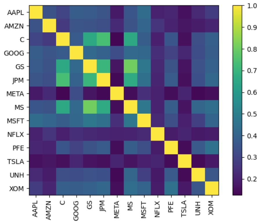
We can implement the aforementioned expected return models as detailed below. We can also plot the calculated covariance estimations and compare them with the real future covariance matrix, in order to observe which covariance estimator performs best:
    from pyfinpo.input_estimates import risk_models

    cov_matrix = risk_models.sample_cov(prices)
    po_plotting.plot_covariance(sample_cov, plot_correlation=True)
    plt.show()
Quick Example:
3.1.2
___ INPUT ESTIMATE 2
Expected
Return Models
Risk
Models
__ PYFINPO FEATURE II
3.2
Portfolio
Optimization
__ Portfolio Optimization I
3.2.1
PO Models
The Portfolio Optimization Model of choice will determine the strategy to follow in the rest of the portfolio optimization process. It dictates how we are approaching the PO problem.
__ Portfolio Optimization II
3.2.2
PO Objectives
The Portfolio Optimization Objectives will define the metric for which we want to optimize the portfolio allocation process. PyFinPo offers several options for risk/return metrics.
__ Portfolio Optimization IV
3.2.4
PO Period
Portfolio Optimization Period defines the Investment Horizon of choice for the optimization, and formulates the problem based on a discrete or continuous time approach.
__ Portfolio Optimization V
3.2.5
PO Solver
Finally, the last step of the Portfolio Optimization process defines the solver (optimizer) to address the actual optimization problem.
3.2
__ Portfolio Optimization III
3.2.3
PO Constraints
The Portfolio Optimization Constraints define the conditions and rules that will govern the Optimization problem.
I) Naive PO Models
| Model Tag | Model Name | Documentation | Code |
|---|---|---|---|
mr_po |
Mean-Risk Portfolio Optimization (generalizes all models below) | skfolio | To be implemented |
mv_po |
Mean-Variance Portfolio Optimization | PyPortOpt | mv_po.py |
msv_po |
Mean-Semivariance Portfolio Optimization | PyPortOpt | msv_po.py |
mcvar_po |
Mean-CVaR (Conditional Value at Risk) Portfolio Optimization | PyPortOpt | mcvar_po.py |
mcdar_po |
Mean-CDaR (Conditional Drawdown at Risk) Portfolio Optimization | PyPortOpt | mcdar_po.py |
List of Risk Measures Supported under MeanRiskPO class:
Mean Absolute Deviation
Variance (Second Central Moment)
Skewness (Normalized Third Central Moment)
Kurtosis (Normalized Fourth Central Moment minus 3)
Fourth Central Moment
First Lower Partial Moment
Semi-Variance (Second Lower Partial Moment)
Fourth Lower Partial Moment
Value at Risk
Maximum Drawdown
___ PORTFOLIO OPTIMIZATION I
Portfolio
Optimization Models
The first step of the portfolio optimization is to choose the optmization model/framework. The model of choice is going to determine the type of approach we want for the portfolio optimization, the different objective functions that we will be able to optimize for, and the solver used to approach the optimization problem, among other things. As we will see later on, each optimization model/framework has its particular objective functions and solvers/optimizers.
The following Portfolio Optimization Models have been/will be implemented:
___ PORTFOLIO OPTIMIZATION II
Portfolio
Average Drawdown
Drawdown at Risk
Entropic Risk Measure
CVaR (Conditional Value at Risk)
EVaR (Entropic Value at Risk)
CDaR (Conditional Drawdown at Risk)
EDaR (Entropic Drawdown at Risk)
Worst Realization
Ulcer Index
Gini Mean Difference
Optimization Objectives
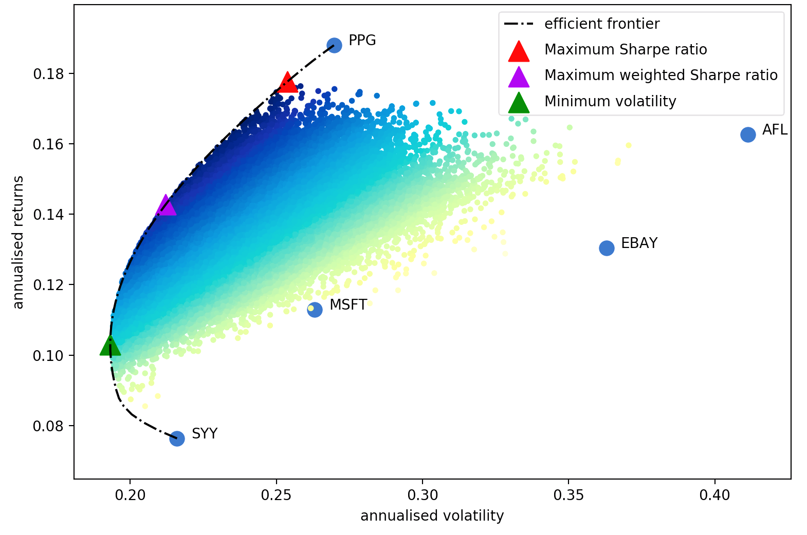
Figure 2 - Mean-Variance Efficient Frontier. Source: PyPortOpt
I) Objective Functions
Some of the Portfolio Optimization Models exposed above are self-descriptive, in the sense that by definition they only posses a single possible objective function to optimize. In these cases, the default objective function will be automatically chosen by the code implementation, and the user will not need to specify any objective.
However, there are other models (the most obvious kind being Mean-Risk models) which allow to select different objective functions to optimize for. The easiest way to picture this behavior is with Mean-Variance theory as an example (see Figure 2). Within the MVT framework we can define the Efficient Frontier, which represents a Pareto Optimal set of possible optimal portfolios.For a given Efficient Frontier, different points can be selected as optimal under different objective functions.
In this context, PyFinPO provides five main objective functions:
Minimum Risk -
global_min_riskRepresents the point of the Optimal Set with lowest level of risk. Its calculation can be useful to have an idea of how low risk could be for a given problem/portfolio.
Minimize Risk -
min_riskMinimizes risk for a given level of return.
Maximize Return -
max_returnMinimizes return for a given level of risk.
Maximize Ratio -
max_ratioMaximizes the ratio return-risk for the whole portfolio. This returns the tangency portfolio, as it represents the point on a returns-risk graph where the tangent to the efficient frontier intersects the y-axis at the risk-free rate. This is the default choice as it finds the optimal return per level of risk at portfolio level.
Maximize Utility -
max_returnMaximizes the utility function provided manually by the user, which specifies its level of risk aversion.
Once again, the word "risk" can be replaced for any of the available risk metrics defined under MeanRiskPO class (see list above).
Note: not all of these objective functions may be available for all the different Mean-Risk models.
II) Adding Custom Objectives
In addition, sometimes we may want to add extra optimization objectives that are not defined in the previous 5 objective functions.
PyFinPO supports the addition of extra optimization objectives. Note that there are 2 types of objectives, convex and non-convex. While convex objectives fit nicely under a convex optimization solver, non-convex objectives may be treated with care as they may produce incompatibilities with the solvers implemented in this library.
Convex Objectives:
L2 regularisation (minimising this reduces nonzero weights)
Transaction cost model (can be added also as constraint)
Custom convex objectives (must be expressed with
cvxpyatomic functions)
Non-Convex Objectives:
See example in the original docs of the PyPortOpt library here
For an example on how to implement custom objectives, see PyFinPO-UserGuide.
III) Single-Objective vs Multi-Objective Optimization
Note that when we provide an specific objective function or set of objectives for the portfolio optimization, it will return a single solution (i.e. single set of optimal weights that represent the optimal portfolio).
Alternatively, we can change our approach and implement a multi-objective optimization where we obtain an optimal set of solutions from which we can choose the preferred one for our objectives. A way to do this, is by plotting the optimal set of solutions (e.g. efficient frontier in case of Mean-Variance Theory) and then choosing the desired portfolio.
___ PORTFOLIO OPTIMIZATION III
Portfolio
Optimization Constraints
3.2.1
Constraints and objectives are treated similarly from an optimization point of view. Therefore, the methodology to add constraints to a portfolio optimization is almost equivalent to the process of adding objectives described above.
The main portfolio optimization constraints available in PyFinPO are:
Market Neutrality
Long/Short Portfolio
Weight Bounds (limit the position size of securities)
Sector & Security Constraints
Score Constraints
Nº of Asset Constraints (Convexity Constraints)
Tracking Error Constraints
For examples on how to implement custom objectives in PyFinPO, see PyFinPO-UserGuide.
II) Risk-Based PO Models
| Model Tag | Model Name | Documentation | Code |
|---|---|---|---|
gmv_po |
Global Minimum Variance PO | PyPortOpt, GMVP | To be implemented |
maxdiv_po |
Maximum Diversification Portfolio Optimization | skfolio | To be implemented |
risk_parity_po |
Risk Parity Portfolio Optimization | skfolio, Risk Parity PO | To be implemented |
risk_budgeting_po |
Risk Budgeting Portfolio Optimization | skfolio, Risk Budgeting PO | To be implemented |
III) Mean-Risk PO Models
Mean-Risk Portfolio Optimization models aim to find asset combinations which optimize the relationship return vs risk. The most well-known Mean-Risk model is Mean-Variance Portfolio Optimization, which uses the variance of asset returns as measure of risk. However, many different measures of risk can be selected, giving rise to a wide range of Mean-Risk models.
PyFinPO provides direct implementation of the most relevant Mean-Risk models, as detailed in the summary table below (Mean-Variance, Mean-Semivariance, Mean-CVaR, Mean-CDaR). In order to select any other measure of risk which is not directly implemented in the PO models below, the parent class MeanRiskPO generalizes all mean-risk models and allows to choose among any of the available risk metrics:
IV) Robust Mean-Risk PO Models
V) Clustering PO Models
VI) Ensemble PO Models
| Model Tag | Model Name | Documentation | Code |
|---|---|---|---|
stack_po |
Stacking Portfolio Optimization | - | To be implemented |
___ PORTFOLIO OPTIMIZATION IV
Portfolio
Optimization Period
One of the main limitations of PyFinPO and most other Portfolio Optimization libraries is that the optimization is static (single-period), meaning that based on the input parameters the output optimal portfolio is only valid for a static period of time. Of course, due to the dynamic nature of financial markets it would be preferable to have a dynamic optimization in order to reflect the latest information available in the optimized portfolio and take optimal rebalancing decisions.
Future development plans for PyFinPO include extending the optimization functionalities to address the portfolio optimization problem dynamically. Two main approaches can be found in literature that address PO dynamically, as a Multi-Period Portfolio Optimization (MPPO):
The first approach considers a discrete-time PO, where the expected utility of the investor terminal wealth is maximized over a multi-period investment horizon, and portfolio can be rebalanced only at discrete points in time (e.g. for a 1-year PSP, adjusting portfolio weights at the beginning of every month).
The second approach is a continuous-time optimization, where asset weights can be reallocated at any time within the investment horizon.
Zhang et. al. provide a detailed review on the formulation and advantages of dynamic PO techniques.
___ PORTFOLIO OPTIMIZATION V
Portfolio
3.2.3
3.2.4
3.2.5
Optimization Solver (Optimizer)
3.2.2
The solver implemented to address the optimization problem in the previous examples has been implemented under the hood of the MeanVariancePO class, which inherits its methods from the BaseConvexOptimizer class. In the context of Mean-Variance theory, as the optimization problem is typically convex (unless non-convex constraints or objectives are introduced), it can be solved via quadratic programming with the cvxpy python library for convex optimization.
While Mean-Variance optimization framework can be addressed with convex optimization, other portfolio optimization models which are completely different in character may use different optimization schemes. An overall summary is presented below for quick reference, including only the main portfolio optimization models and the optimization solver they use in this library.
| Portfolio Optimization Model | Module | Main Class | Optimization Solver | Optimization Solver Details |
|---|---|---|---|---|
| Mean-Variance Portfolio Optimization | mv_po.py |
MeanVariancePO |
BaseConvexOptimizer |
MVPO is addressed with convex optimization via cvxpy |
| Mean-SemiVariance Portfolio Optimization | msv_po.py |
MeanSemivariancePO |
BaseConvexOptimizer |
MSVPO can be re-written as convex problem (full details here) |
| Mean-CVaR Portfolio Optimization | mcvar_po.py |
MeanCVaRPO |
BaseConvexOptimizer |
MCVaRPO can be reduced to linear program (full details here) |
| Mean-CDaR Portfolio Optimization | mcdar_po.py |
MeanCDaRPO |
BaseConvexOptimizer |
MCDaRPO can be reduced to linear program (full details here) |
| Critical Line Algorithm Portfolio Optimization | cla_po.py |
CLAPO |
BaseOptimizer |
CLAPO uses CLA convex optimization solver, specifically designed for PO |
| Hierarchical Risk Parity Portfolio Optimization | hrp_po.py |
HRPPO |
BaseOptimizer |
HRPPO implements hierarchical clustering optimization (more details here) |
*For a more detailed analysis on how to choose the right solver for any risk metric, visit Riskfolio-Lib - Choosing a Solver.
__ PYFINPO FEATURE III
3.3
Portfolio Performance
The Portfolio Performance module is a key component of the portfolio optimization repository, designed to evaluate and analyze the effectiveness of optimized portfolios. It is in charge of computing essential performance metrics such as expected annual return, volatility (risk), and Sharpe Ratio, providing a comprehensive view of portfolio performance. These metrics help investors assess the trade-off between risk and return, ensuring that the portfolio aligns with their investment goals. By leveraging this module, users can make data-driven decisions and refine their strategies for better financial outcomes. The module is flexible, easy to integrate, and supports various portfolio optimization models.
3.3
__ PYFINPO FEATURE III
3.4
Portfolio
Post-Processing
__ Post-Processing I
3.4.1
Portfolio
(Tidy) Weights
Express portfolio optimal weights in a more visual, tidy way.
__ Post-Processing II
3.4.2
Portfolio
Discrete Allocation
Express portfolio weights in execution terms (how much quantity of each stock to buy at the current market price).
3.4
___ PORTFOLIO POST-PROCESSING I
Portfolio
3.4.1
    mv_po = po_models.MeanVariancePO(mhr, sample_cov, weight_bounds=(0,1))

    mv_po.min_volatility()
    optimal_portfolio_clean_weights = mv_po.clean_weights()
    optimal_portfolio_clean_weights
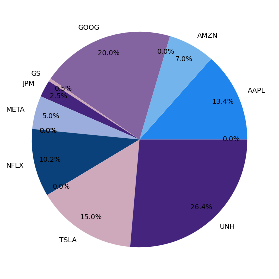
pd.Series(mv_po).plot.pie(figsize=(7,7), colors=colors, autopct='%1.1f%%', pctdistance=0.85)
(Tidy) Weights
PyFinPo also offers the option to express portfolio optimal weights in a more visual, tidy way with the .clean_weights() method (see PyFinPO-UserGuide).
___ PORTFOLIO POST-PROCESSING II
Portfolio
3.4.2
Discrete Allocation
Once we have the optimal portfolio weights, it is probably useful to express it in execution terms (how much quantity of each stock to buy at the current market price). The function discrete_allocation helps us with this purpose:
    from pyfinpo.utils import DiscreteAllocation

    latest_prices = prices.iloc[-1]  # prices as of the day you are allocating
    da = DiscreteAllocation(optimal_portfolio_weights, latest_prices,
                            total_portfolio_value=20000, short_ratio=0.3)
    alloc, leftover = da.lp_portfolio()
    print(f"Discrete allocation performed with ${leftover:.2f} leftover")
    {key: float(value) for key, value in alloc.items()}
    #Output:


    Discrete allocation performed with $13.46 leftover
    {'AAPL': 3.0,
     'GOOG': 8.0,
     'META': 5.0,
     'MSFT': 3.0,
     'PFE': 218.0,
     'TSLA': 2.0,
     'UNH': 4.0,
     'XOM': 46.0}
04
Future Works/Resources __________
Future Works & Resources
Chapter 4 -
3.3
Future
Works
Some of the improvements that may be added in future versions of PyFinPO include the following:
Develop detailed documentation for models and API usage under
docsfolder.Finish implementation of all the return models, risk models and portfolio optimization models whose status appears as "To be implemented" in the summary tables described above.
Include the implementation of multi-period optimization. See more details in Section 3.2.4.
Improve Portfolio Performance function to depict a more detailed analysis about the optimized portfolio, including additional measures of risk, performance ratios, backtesting functionalities, sensitivity analysis...
Implement tests for all library functionalities under the folder
tests.Add additional tutorials under the folder
tutorials(currently only 2 are available) to cover more practical use cases of different optimizations and functionalities that can be performed withPyFinPO.
Source
Libraries
PyFinPO is an abstraction built on top of the following Python libraries:
SEE MORE PROJECTS

MATH, PHYSICS & ENGINEERING PROJECTS

COMPUTER SCIENCE PROJECTS

ML & AI PROJECTS

QUANT FINANCE PROJECTS